Chapter 5 Notes
Correlation
Correlation is very common, and in large data sets, pretty much every variable is correlated to some degree. Since correlations do not indicate causal relationships, we need a way to distinguish association from evidence of causation.
Multivariate regression is one such tool for this and there are several reasons why they are popular.
They allow for “control” for confounds. A confound is a variable which has no real importance, but because of it’s correlation might appear important. Be careful though! Confounds can hide real important variables just as easily as they can produce false ones. Simpson’s Paradox found that the entire direction of an apparant association between a predictor and outcome can be reversed by considering a confound.
Multiple causation. Even when confounds are absent, it is entirely possible that phenomenon may arise from multiple causes. When causation is multiple, one cause can hide another.
Interactions. Even when variables are completely uncorrelated, the importance of each may still depend upon the other. For example, plants benefit from both light and water, but if either were abscent, there would be no benefit at all.
Spurious association
Let’s consider divorce rates with the following linear regression model.
\[ \begin{array}{l} D_{i} \sim \text{Normal}(\mu_{i}, \sigma) \\ \mu_{i} = \alpha + \beta_{A}A_{i} \\ \alpha \sim \text{Normal}(10, 10) \\ \beta_{A} \sim \text{Normal}(0, 1) \\ \sigma \sim \text{Uniform}(0, 10) \end{array} \]
- \(D_{i}\) is the divorse rate for State \(i\).
- \(A_{i}\) is State \(i\)’s median age at marriage.
data(WaffleDivorce)
d <- WaffleDivorce

# standardize predictor
d$MedianAgeMarriage.s <- (d$MedianAgeMarriage - mean(d$MedianAgeMarriage))/sd(d$MedianAgeMarriage)

# fit model
m <- quap(
  alist(
    Divorce ~ dnorm(mu, sigma),
    mu <- alpha + beta*MedianAgeMarriage.s,
    alpha ~ dnorm(10, 10),
    beta ~ dnorm(0, 1),
    sigma ~ dunif(0, 10)
  ), data = d)

precis(m)
## mean sd 5.5% 94.5%
## alpha 9.688224 0.2045084 9.361380 10.0150679
## beta -1.042823 0.2025347 -1.366513 -0.7191339
## sigma 1.446395 0.1447674 1.215029 1.6777614# sd(d$MedianAgeMarriage)
# 1.24
# compute percentile interval of mean
MAM.seq <- seq(from = -3, to = 3.5, length.out = 30)
mu <- link(m, data = data.frame(list(MedianAgeMarriage.s = MAM.seq)))
mu.PI <- apply(mu, 2, PI)
# plot it all
plot(Divorce ~ MedianAgeMarriage.s, data = d, col = rangi2)
abline(m)
shade(mu.PI, MAM.seq)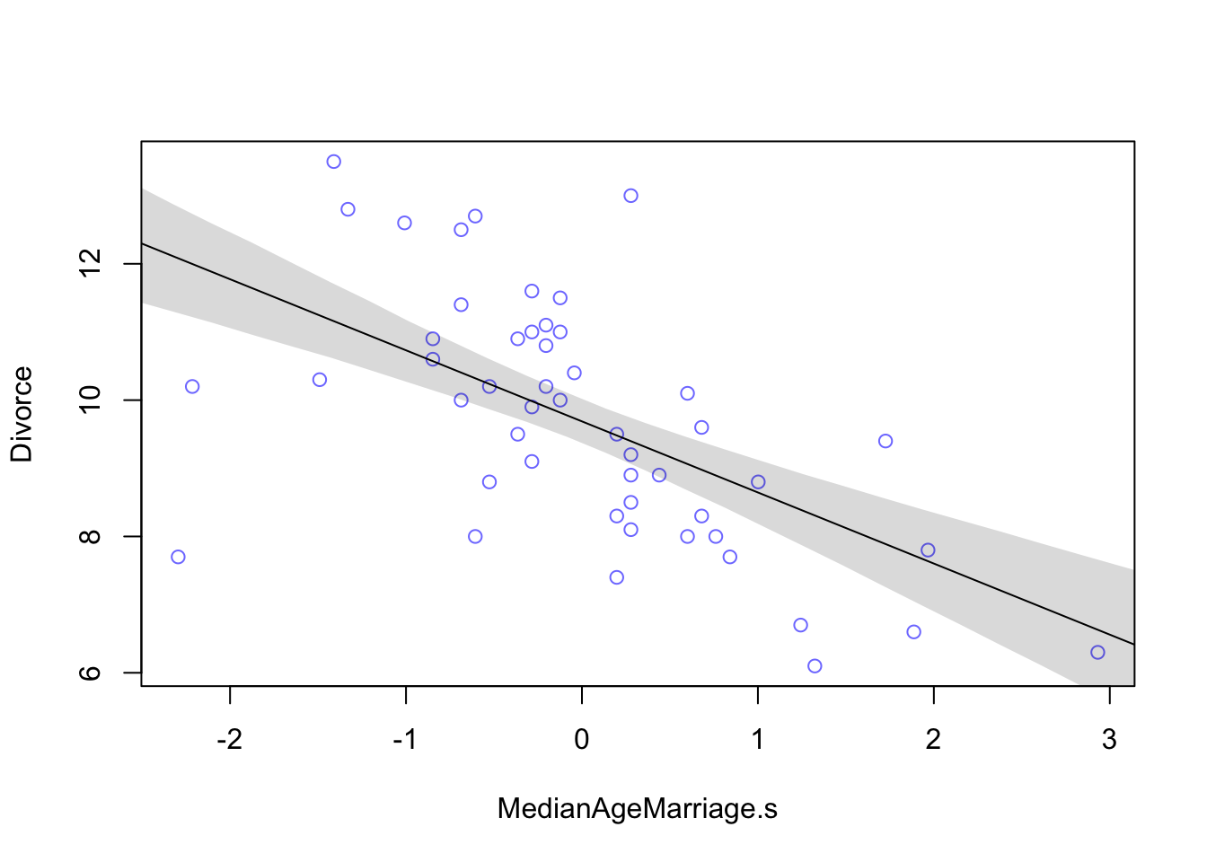 From the table we can see that for each additional standard deviation of delay in marriage (1.24 years), predicts a decrease of about one divorce per thousand adults with a 89% interval from about -1.37 to -0.72. Even though the magnitude may vary a lot, we can still say that it’s reliably negative.
d$Marriage.s <- (d$Marriage - mean(d$Marriage))/sd(d$Marriage)
m2 <- quap(
  alist(
    Divorce ~ dnorm(mu, sigma),
    mu <- alpha + beta*Marriage.s,
    alpha ~ dnorm(10, 10),
    beta ~ dnorm(0, 1),
    sigma ~ dunif(0, 10)
  ), data = d)

precis(m2)
## mean sd 5.5% 94.5%
## alpha 9.6881748 0.2364320 9.3103108 10.066039
## beta 0.6437544 0.2324645 0.2722313 1.015278
## sigma 1.6722941 0.1673041 1.4049099 1.939678# sd(d$Marriage)
# 3.8
# compute percentile interval of mean
Marriage.seq <- seq(from = -3, to = 3.5, length.out = 30)
mu2 <- link(m2, data = data.frame(list(Marriage.s = Marriage.seq)))
mu2.PI <- apply(mu2, 2, PI)
# plot it all
plot(Divorce ~ Marriage.s, data = d, col = rangi2)
abline(m2)
shade(mu2.PI, Marriage.seq)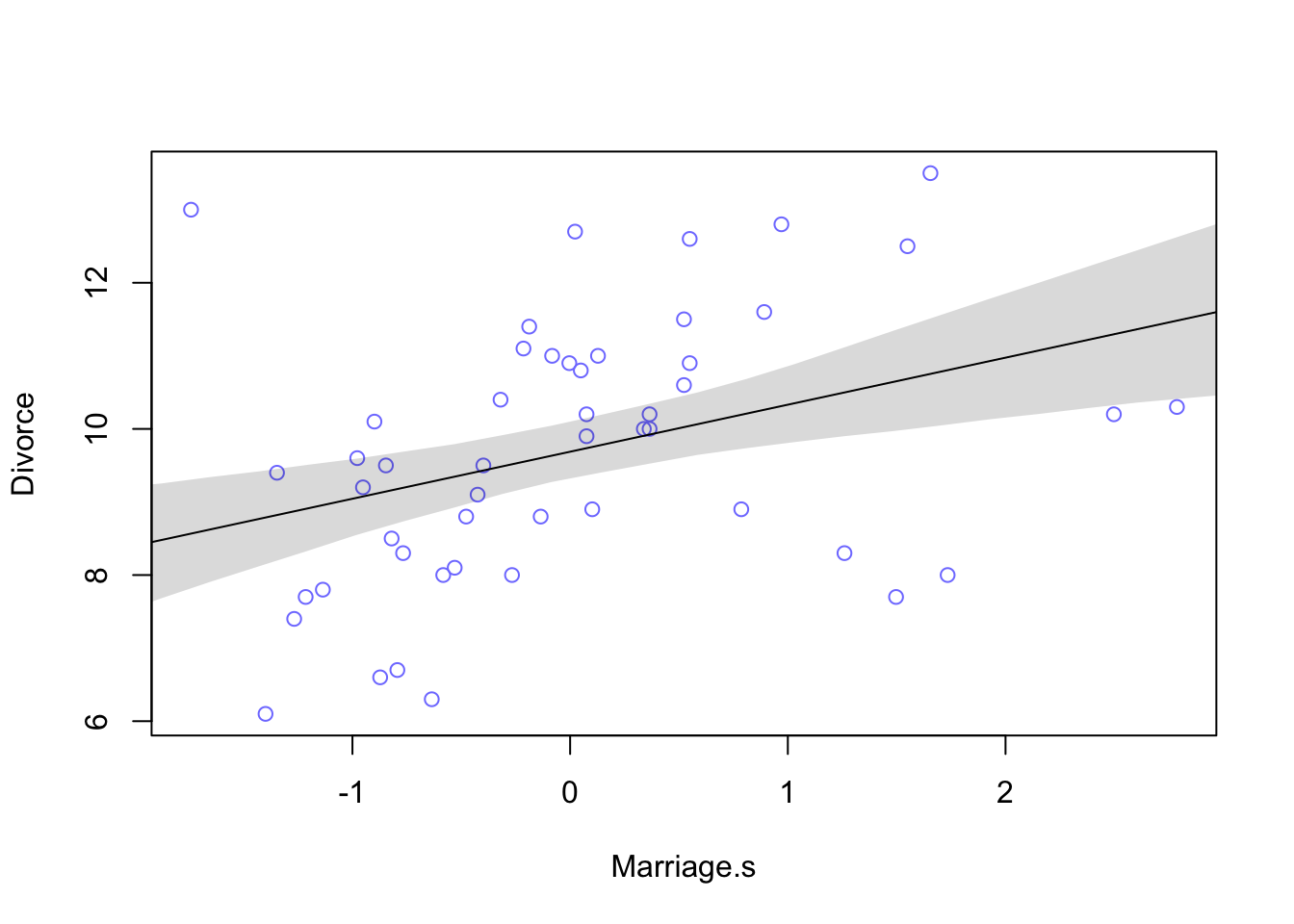
The table output shows that for every additional standard deviation of marriage rate (3.8), there is an increase of 0.6 divorces. Looking at the plot we can see that this relationship isn’t as strong as the previous one.
What is the predictive value of a variable, once I already know all the other predictor variables?
Once we fit a multivariate model to predict divorce using both marriage rate and age at marriage, the model will answer the following:
- After we already know marriage rate, what additional value is there in also knowing age at marriage?
- Afte we already know age at marriage, what additional value is there in also knowing marriage rate?
Multivariate Notation
If we want a model that predicts divorce rate using both marriage rate and age at marriage, the methods are very similar to how we defined polynomial models before:
- Select the predictor variables you want in the linear model of the mean
- For each predictor, make a parameter that will measure its association with the outcome
- Multiply the parameter by the variable and add that term to the linear model
\[ \begin{array}{lr} D_{i} \sim \text{Normal}(\mu_{i}, \sigma) & \text{[likelihood]} \\ \mu_{i} = \alpha + \beta_{R}R_{i} + \beta_{A}A_{i} & \text{[linear model]}\\ \alpha \sim \text{Normal}(10, 10) & [\text{prior for }\alpha] \\ \beta_{R} \sim \text{Normal}(0,1) & [\text{prior for }\beta_{R}] \\ \beta_{A} \sim \text{Normal}(0, 1) & [\text{prior for }\beta_{A}] \\ \sigma \sim \text{Uniform}(0,10) & [\text{prior for }\sigma] \end{array} \] Here, \(R\), represents the marriage rate and \(A\), the age at marriage. But what does \(\mu_{i} = \alpha + \beta_{R}R_{i} + \beta_{A}A_{i}\) mean? It means the expected outcome for any State with marriage rate \(R_{i}\) and meadian age at marriage \(A_{i}\) is the sum of three independent terms. An easier way to interpret this would be: A State’s divorce rate can be a function of its marriage rate or its median age at marriage.
# Now fitting the model in R
m <- quap(
  alist(
    Divorce ~ dnorm(mu, sigma),
    mu <- alpha + betaR*Marriage.s + betaA*MedianAgeMarriage.s,
    alpha ~ dnorm(10, 10),
    betaR ~ dnorm(0, 1),
    betaA ~ dnorm(0, 1),
    sigma ~ dunif(0, 10)
  ), data = d)

knitr::kable(cbind(precis(m), cov2cor(vcov(m))), digits = 2)| mean | sd | 5.5% | 94.5% | alpha | betaR | betaA | sigma | |
|---|---|---|---|---|---|---|---|---|
| alpha | 9.69 | 0.20 | 9.36 | 10.01 | 1 | 0.00 | 0.00 | 0.00 |
| betaR | -0.13 | 0.28 | -0.58 | 0.31 | 0 | 1.00 | 0.69 | 0.05 |
| betaA | -1.13 | 0.28 | -1.58 | -0.69 | 0 | 0.69 | 1.00 | 0.07 |
| sigma | 1.44 | 0.14 | 1.21 | 1.67 | 0 | 0.05 | 0.07 | 1.00 |
The posterior mean for marriage rate, \(\beta_{R}\), is now close to zero, with plenty of probability on both sides of zero. The posterior mean for age at marriage, \(\beta_{A}\), has actually gotten slightly farther from zero but is essentially unchanged.
plot(precis(m))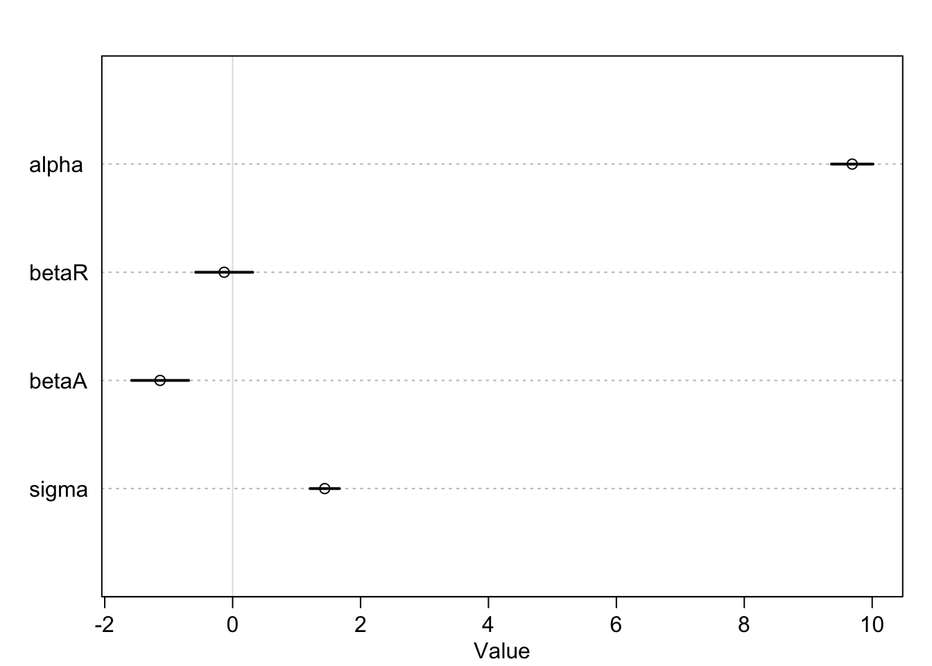
Interpretation: Once we know median age at marriage for a State, there is little or no additional predictive power in also knowing the rate of marriage in that State.
Plotting mutlivariate posteriors
Plotting multiple linear regression is difficult because it requires a lot of plots, and most do not generalize beyond linear regression. Instead, we’ll focus on three types of interpretive plots:
- Predictor residual plots. These plots show the outcome against residual predictor values. It’s probably not recommended to use this method moving forward, however, it’s a good way to visualize what the multivariate regression is doing underneath the hood.
- Counterfactual plots. These show the implied predictions for imaginary experiments in which the different predictor variables can be changed independently of one another.
- Posterior prediction plots. These show model-based predictions against raw data, or otherwise display the error in prediction.
Predictor residual plots
In our multivariate model of divorce rate, we have two predictors (1) marriage rate (Marriage.s) and (2) median age at marriage (MedianAgeMarriage.s). To compute predictor residuals for either, we just use the other predictor to model it. So for marriage rate, this is the model we need.
\[ \begin{array}{l} R_{i} \sim \text{Normal}(\mu, \sigma) \\ \mu_{i} = \alpha + \beta A_{i} \\ \alpha \sim \text{Normal}(0, 10) \\ \beta \sim \text{Normal}(0,1) \\ \sigma \sim \text{Uniform}(0,10) \end{array} \]
As before, \(R\) is marriage rate and \(A\) is median age at marriage. Since we standardized both variables, we already expect the mean \(\alpha\) to be around zero, which is why we’ve centered \(\alpha\)’s prior there.
m <- quap(
  alist(
    Marriage.s ~ dnorm(mu, sigma),
    mu <- alpha + beta*MedianAgeMarriage.s,
    alpha ~ dnorm(0, 10),
    beta ~ dnorm(0, 1),
    sigma ~ dunif(0, 10)
  ), data = d)
Now that we have the model, we compute the residuals by subtracting the observed marriage rate in each State from the predicted rate, based upon using age at marriage.
# compute expected value
mu <- coef(m)['alpha'] + coef(m)['beta']*d$MedianAgeMarriage.s

# compute residual for each State
m.resid <- d$Marriage.s - mu
d %>%
ggplot(aes(x = MedianAgeMarriage.s, y = Marriage.s)) +
geom_point(size = 2, shape = 1, color = "royalblue") +
geom_segment(aes(xend = MedianAgeMarriage.s, yend = mu), size = 1/4) +
geom_line(aes(y = mu)) +
coord_cartesian(ylim = range(d$Marriage.s)) +
theme_bw() +
theme(panel.grid = element_blank())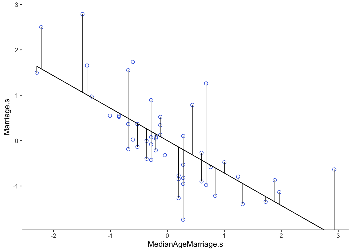
From here we would say that States with a positive residual marry fast for their age of marriage, while States with negative residuals marry slow for their age of marriage.
# make a data frame for ggplot
r <- m.resid %>%
  as.data.frame() %>%
  cbind(d)

# Create a predictor residual plot
prp1 <-
  r %>%
  ggplot(aes(x = m.resid, y = Divorce)) +
  geom_smooth(method = 'lm', formula = y ~ x,
              fullrange = TRUE,
              color = "grey", fill = "grey",
              alpha = 1/5, size = 1/2) +
  geom_vline(xintercept = 0, linetype = 2, color = "grey50") +
  geom_point(size = 2, color = "royalblue", alpha = 2/3) +
  annotate("text", x = c(-0.35, 0.35), y = 14.1, label = c("slower", "faster")) +
  scale_x_continuous("Marriage rate residuals", limits = c(-2, 2)) +
  coord_cartesian(xlim = range(m.resid),
                  ylim = c(6, 14.1)) +
  theme_bw() +
  theme(panel.grid = element_blank())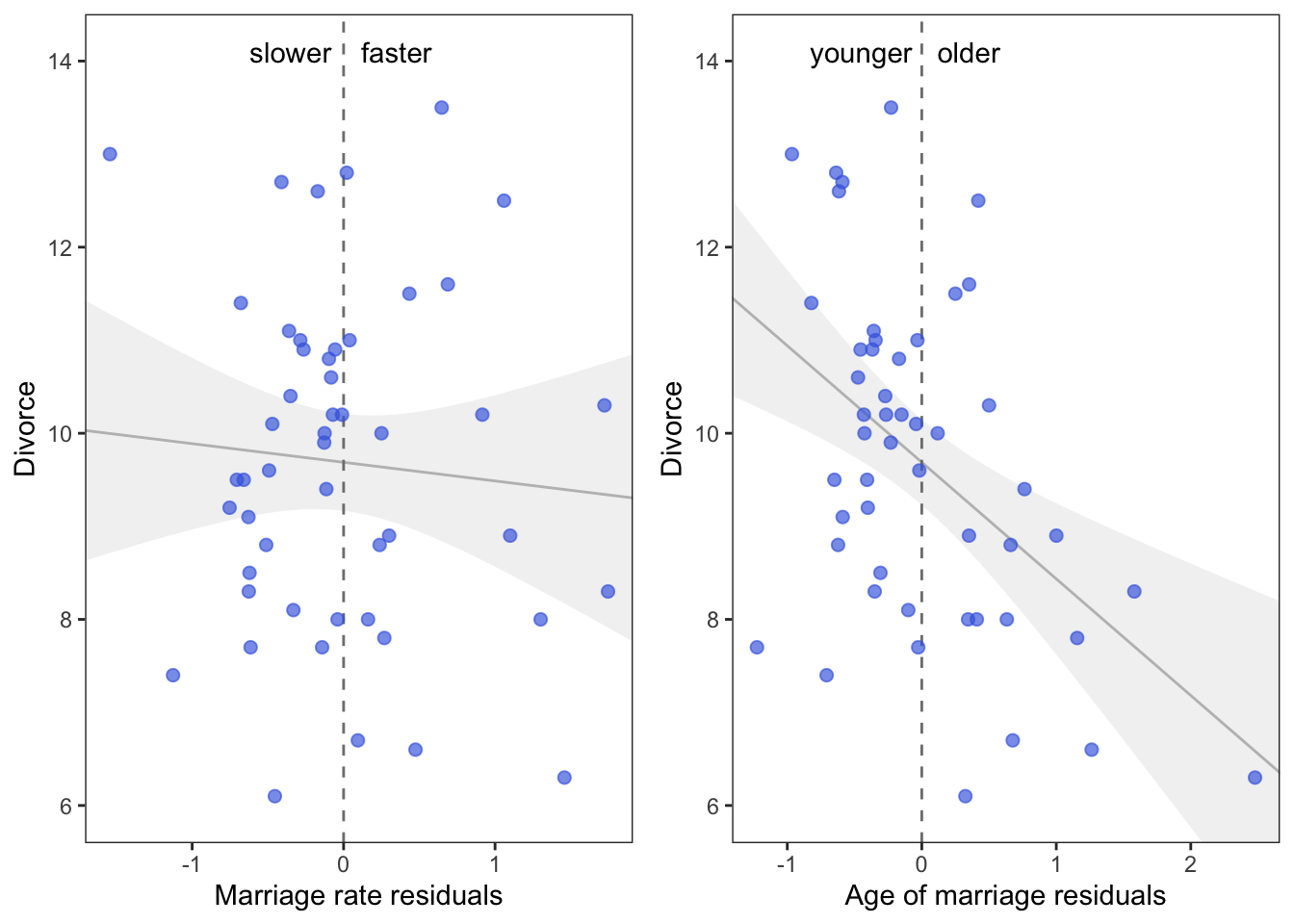
Interpretation: On the left we see that States with fast marriage rates for their median age of marriage have about the same divorce rates as States with slow marriage rates. On the right we see that States with an older median age of marriage for their marriage rate have lower divorce rates than States with a younger median age of marriage.
This is all a visual representation of what we saw when we made our multivariate model above, the slope of the regression lines are identical.
dagify(D ~ A + M,
       M ~ A,
       labels = c("D" = "Divorce",
                  "A" = "Age of marriage",
                  "M" = "Marriage rate"),

       coords = list(x = c(A = 0, D = 1, M = 2),
                     y = c(A = 1, D = 0, M = 1))) %>%
  ggdag(use_labels = "label") #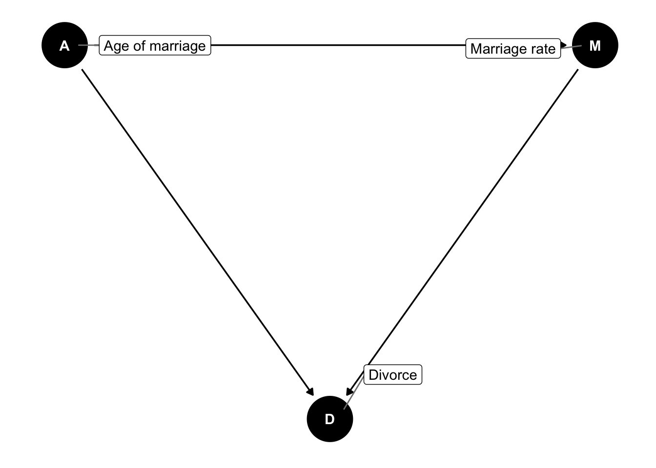
       # labels = c("Divorce" = "Divorce",
       #            "A" = "Age of marriage",
       #            "M" = "Marriage rate"),
Counterfactual plots
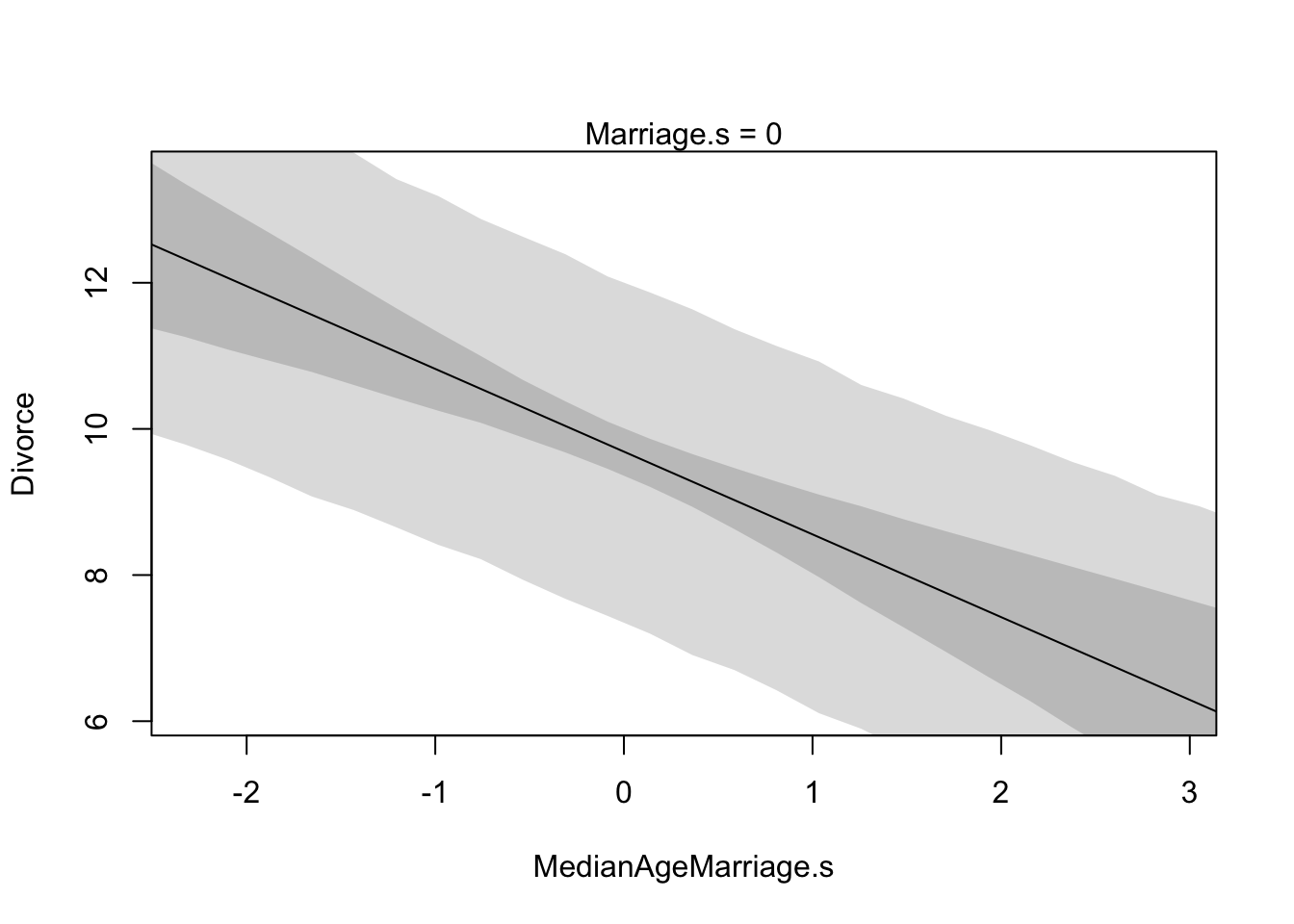
These plots display the implied predicitions of the model. They are called counterfactual, because they can be used to visualize unobserved or even impossible combinations of predictor variables, such as a very high median age of marriage and very high marriage rate. The simplest use case is to see how predictions change as we modify only one predictor at a time. This will help us understand the implications of the model.
# prepare new counterfactual data
A.avg <- mean(d$MedianAgeMarriage.s)
R.seq <- seq(from = -3, to = 3, length.out = 30)
pred.data1 <- data.frame(
  Marriage.s = R.seq,
  MedianAgeMarriage.s = A.avg
)
pred.data <- data.frame(
  Marriage.s = R.seq,
  MedianAgeMarriage.s = A.avg
)

# compute counterfactual mean divorce (mu)

m <- map(
    alist(
        Divorce ~ dnorm(mu, sigma),
        mu <- alpha + betaR*Marriage.s + betaA*MedianAgeMarriage.s ,
        alpha ~ dnorm( 10 , 10 ) ,
        betaR ~ dnorm( 0 , 1 ) ,
        betaA ~ dnorm( 0 , 1 ) ,
        sigma ~ dunif( 0 , 10 )
), data = d )

mu <- link(m, data = pred.data)
mu.mean <- apply(mu, 2, mean)
mu.PI <- apply(mu, 2, PI)

# simulate counterfactual divorce outcomes
R.sim <- sim(m, data = pred.data, n = 1e4)
R.PI <- apply(R.sim, 2, PI)

# display predictions, hiding raw data with type = 'n'
plot(Divorce ~ Marriage.s, data = d, type = "n")
mtext("MedianAgeMarriage.s = 0")
lines(R.seq, mu.mean)
shade(mu.PI, R.seq)
shade(R.PI, R.seq)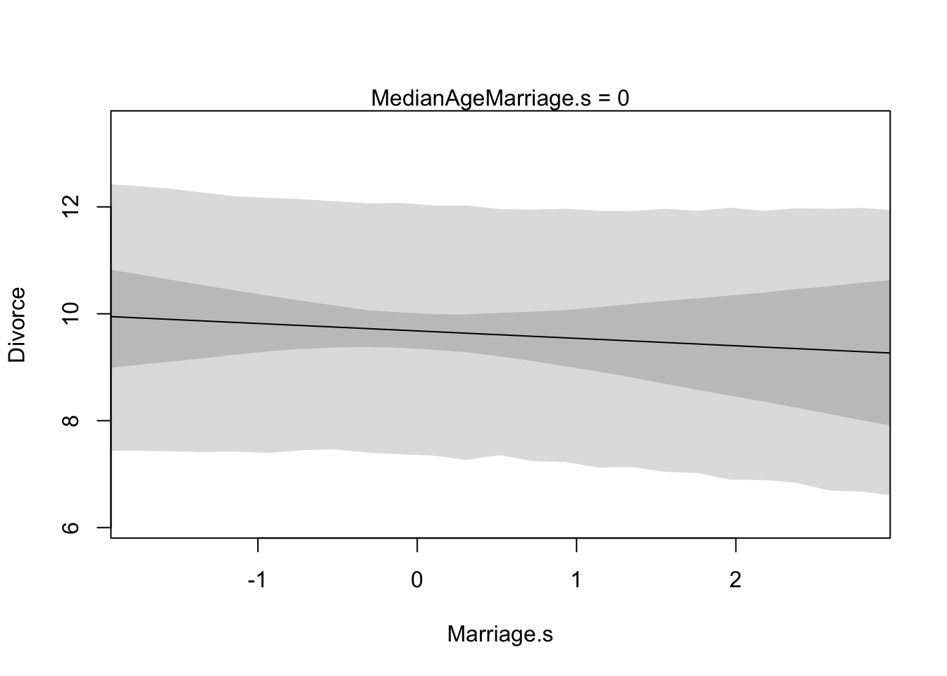
Mitchell Joseph
Data Scientist
My research interests include survival analysis, bayesian statistics, statistical learning, and finance.