Chapter 3 Problem Set
Disclaimer
Below are my solutions to the end of chapter exercises in Statistical Rethinking by Richard McElreath.
These results might not be correct. If you catch any errors or mistakes please leave a comment below.
Easy.
These problems use the samples from the posterior distribution for the globe tossing example. This code will give you a specific set of samples, so that you can check your answers exactly.
p_grid <- seq(from = 0, to = 1, length.out = 1000)
prior <- rep(1, 1000)
likelihood <- dbinom(6, size = 9, prob = p_grid)
posterior <- likelihood * prior
posterior <- posterior/sum(posterior)

set.seed(100)
samples <- sample(p_grid, prob = posterior, size = 1e4, replace = TRUE)
3E1
How much posterior probability lies below p = 0.2?
# sum(posterior[p_grid < 0.2])
sum(samples < 0.2)/1e4
## [1] 5e-04Interpretation: About 0.05% of the posterior probability is below 0.2
3E2
How much posterior probability lies above p = 0.8?
sum(samples > 0.8)/1e4## [1] 0.1117Interpretation: About 11% of the posterior probability is above 0.8
3E3
How much posterior probability lies between p = 0.2 and p = 0.8?
sum(samples > 0.2 & samples < 0.8)/1e4## [1] 0.8878Interpretation: About 89% of the posterior probability is between 0.2 and 0.8
3E4
20% of the posterior probability lies below which value of p?
quantile(samples, 0.2)## 20%
## 0.5195195# Check
sum(samples < 0.5195195)/ 1e4## [1] 0.199720% of the posterior probability lies below p = 0.52
3E5
20% of the posterior probability lies above which value of p?
quantile(samples, 0.8)## 80%
## 0.7567568# Check
sum(samples > 0.7567568)/1e4## [1] 0.198920% of the posterior probability lies above p = 0.757
3E6
Which values of p contain the narrowest interval equal to 66% of the posterior probability?
HPDI(samples, prob = 0.66)## |0.66 0.66|
## 0.5205205 0.7847848# Check
sum(samples > 0.52 & samples < 0.78)/1e4## [1] 0.65273E7
Which values of p contain 66% of the posterior probability, assuming equal posterior probabbility both below and above the interval?
PI(samples, prob = 0.66)## 17% 83%
## 0.5005005 0.76876883M1
Suppose the globe tossing data had turned out to be 8 water in 15 tosses. Construct the posterior distribution, using grid approximation. Use the same flat prior as before.
p_grid <- seq(from = 0, to = 1, length.out = 1000)
prior <- rep(1, 1000)
likelihood <- dbinom(8, size = 15, prob = p_grid)
posterior <- likelihood * prior
posterior <- posterior / sum(posterior)
plot(x = p_grid, y = posterior, type = 'l')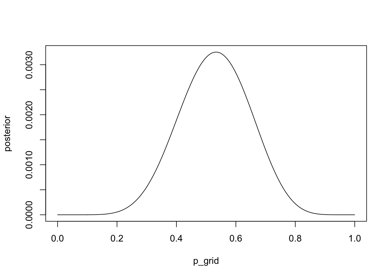
3M2
Draw 10,000 samples from the grid approximation from above. Then use the samples to calculate the 90% HPDI for p.
samples <- sample(p_grid, prob = posterior, size = 1e4, replace = TRUE)

ans_3M2 <- HPDI(samples, prob = 0.90)
ans_3M2
## |0.9 0.9|
## 0.3383383 0.731731790% of the posterior probability is between p=0.33 and p=0.72
3M3
Construct a posterior predictive check for this model and data. This means simulate the distribution of samples, averaging over the posterior uncertainty in p. What is the probability of observing 8 water in 15 tosses.
w <- rbinom(1e4, size = 15, prob = samples)
simplehist(w)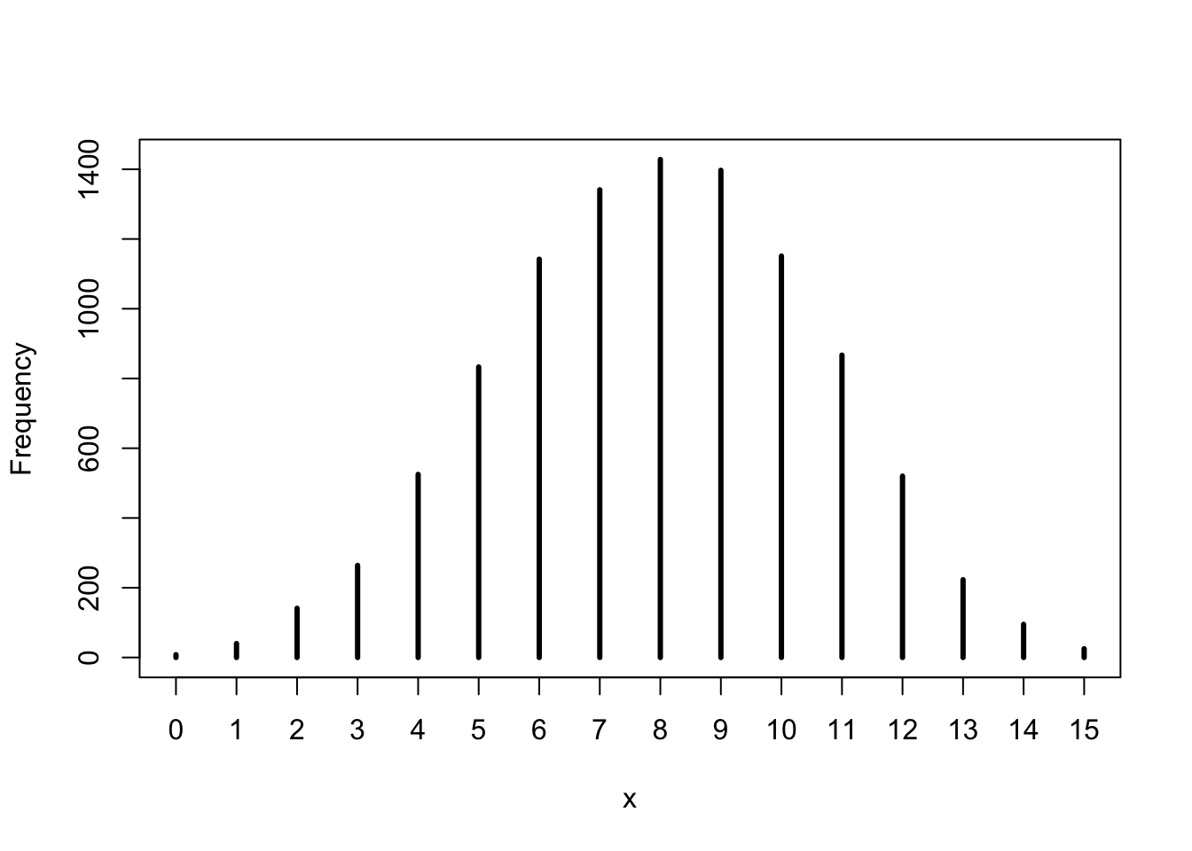
ans_3M3 <- sum(w == 8)/1e4
ans_3M3
## [1] 0.1428# mean(w1 == 8) yields the same result3M4
Using the posterior distribution constructed from the new (8/15) data, now calculate the probability of observing 6 water in 9 tosses.
w <- rbinom(1e4, size = 9, prob = samples)
simplehist(w)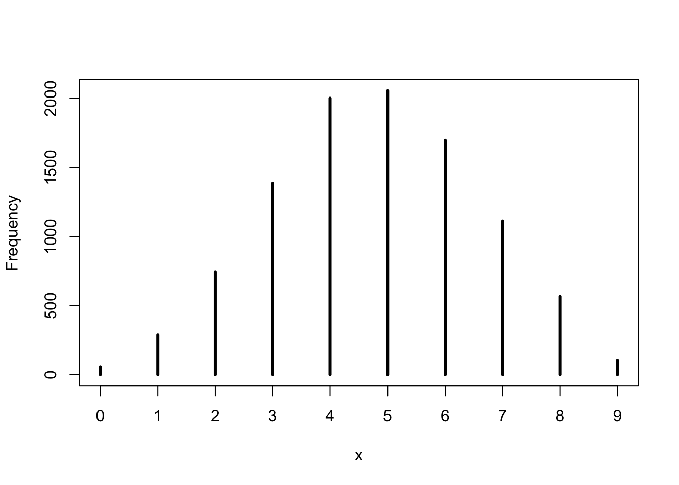
ans_3M4 <- mean(w == 6)
ans_3M4
## [1] 0.16953M5
Start over at 3M1, but now use a prior that is zero below p = 0.5 and a constant above p = 0.5. This corresponds to prior information that a majority of the Earth’s surface is water. Repeat each problem above and compare the inferences. What difference does the better prior make? If it helps, compare inferences (unsing both priors) to the true value p = 0.7.
p_grid <- seq(from = 0, to = 1, length.out = 1000)
prior2 <- ifelse(p_grid < 0.5, 0, 1)
likelihood <- dbinom(8, size = 15, prob = p_grid)
posterior2 <- likelihood * prior2
posterior2 <- posterior2 / sum(posterior2)
plot(x = p_grid, y = posterior2, type = 'l')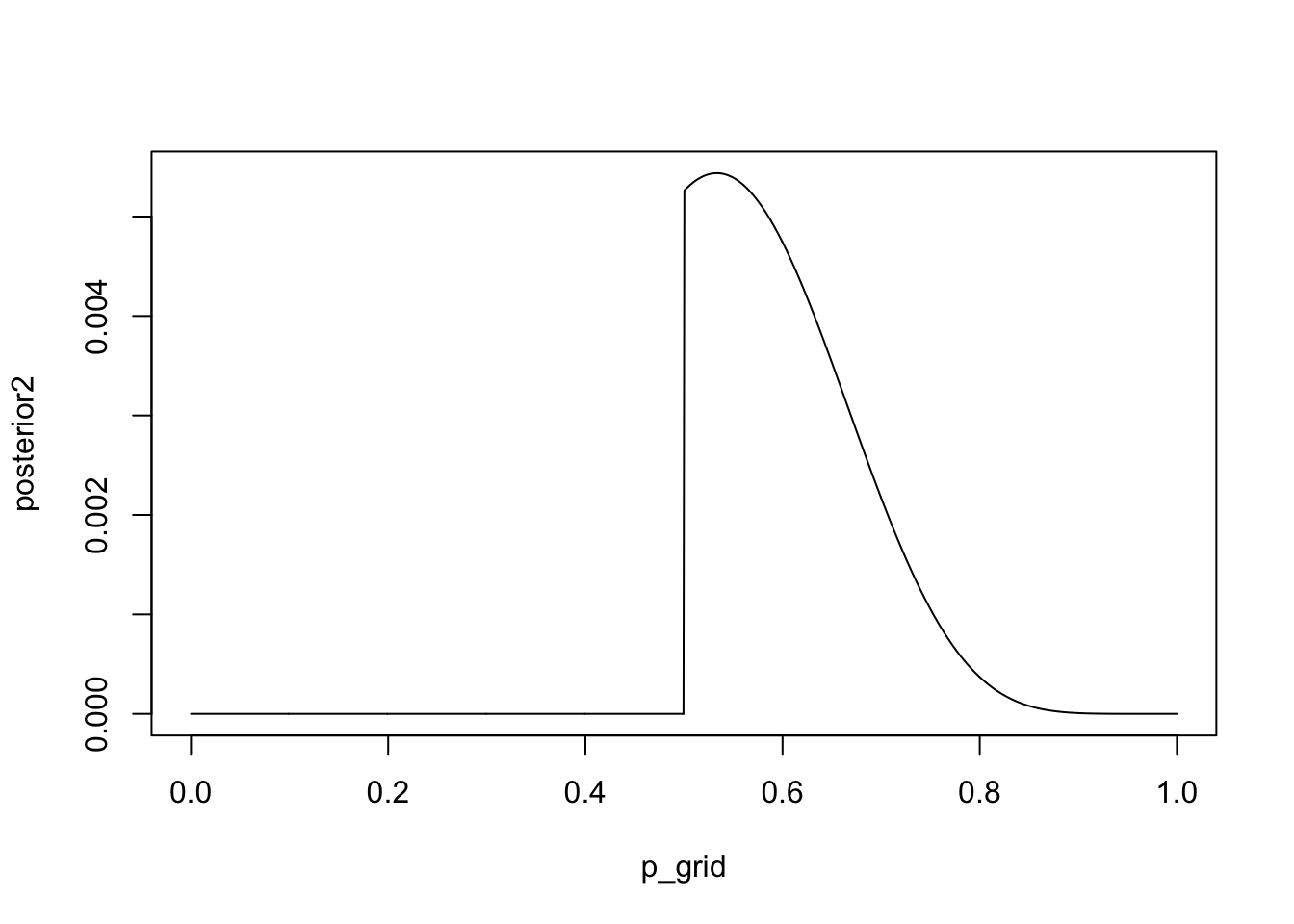
# 3M2
samples2 <- sample(p_grid, prob = posterior2, size = 1e4, replace = TRUE)
ans_3M52 <- HPDI(samples2, prob = 0.90)

# 3M3
w <- rbinom(1e4, size = 15, prob = samples2)
ans_3M53 <- mean(w == 8)

# 3M4
w <- rbinom(1e4, size = 9, prob = samples2)
ans_3M54 <- mean(w == 6)

d <- data.frame("Problem" = c("HPDI lower bound", "HPDI upper bound", "3M3", "3M4"), "Uniform prior" = c(ans_3M2[[1]], ans_3M2[[2]], ans_3M3, ans_3M4), "Updated prior" = c(ans_3M52[[1]], ans_3M52[[2]], ans_3M53, ans_3M54))

knitr::kable(d)| Problem | Uniform.prior | Updated.prior |
|---|---|---|
| HPDI lower bound | 0.3383383 | 0.5005005 |
| HPDI upper bound | 0.7317317 | 0.7097097 |
| 3M3 | 0.1428000 | 0.1592000 |
| 3M4 | 0.1695000 | 0.2357000 |
3H1
The practice problems here all use the data below. These data indicate the gender (male = 1, female = 0) of officially reported first and second born children in 100 two-child families.
data(homeworkch3)
boys <- sum(birth1) + sum(birth2)

p_grid <- seq(from = 0 , to = 1, length.out = 1000)
prior <- rep(1, 1000)
likelihood <- dbinom(boys, size = 200, prob = p_grid)
posterior <- likelihood * prior
posterior <- posterior/sum(posterior)
plot(x = p_grid, y = posterior, type = 'l')
p_grid[which.max(posterior)]## [1] 0.55455463H2
Using the sample function, draw 10,000 random parameter values from the posterior distribution you calculated above. Use these samples to estimate the 50%, 89%, and 97% highest posterior density intervals.
samples <- sample(p_grid, prob = posterior, size = 1e4, replace = TRUE)

HPDI(samples, prob = 0.5)
## |0.5 0.5|
## 0.5255255 0.5725726HPDI(samples, prob = 0.89)## |0.89 0.89|
## 0.5015015 0.6116116HPDI(samples, prob = 0.97)## |0.97 0.97|
## 0.4764765 0.62862863H3
Use rbinom to simulate 10,000 replicates of 200 births. You should end up with 10,000 numbers, each one a count of boys out of 200 births. Compare the distribution of predicted numbers of boys to the actual count in the data (111 boys out of 200 births). There are many good ways to visualize the simulations, but the dens command is probably the easiest way in this case. Does it look like the model fits the data well? That is, does the distribution of predictions include the actual observation as a central, likely outcome?
As we see here, the distribution seems to fit the data fairly well.
w <- rbinom(1e4, size = 200, prob = samples)
dens(w)
abline(v = 111)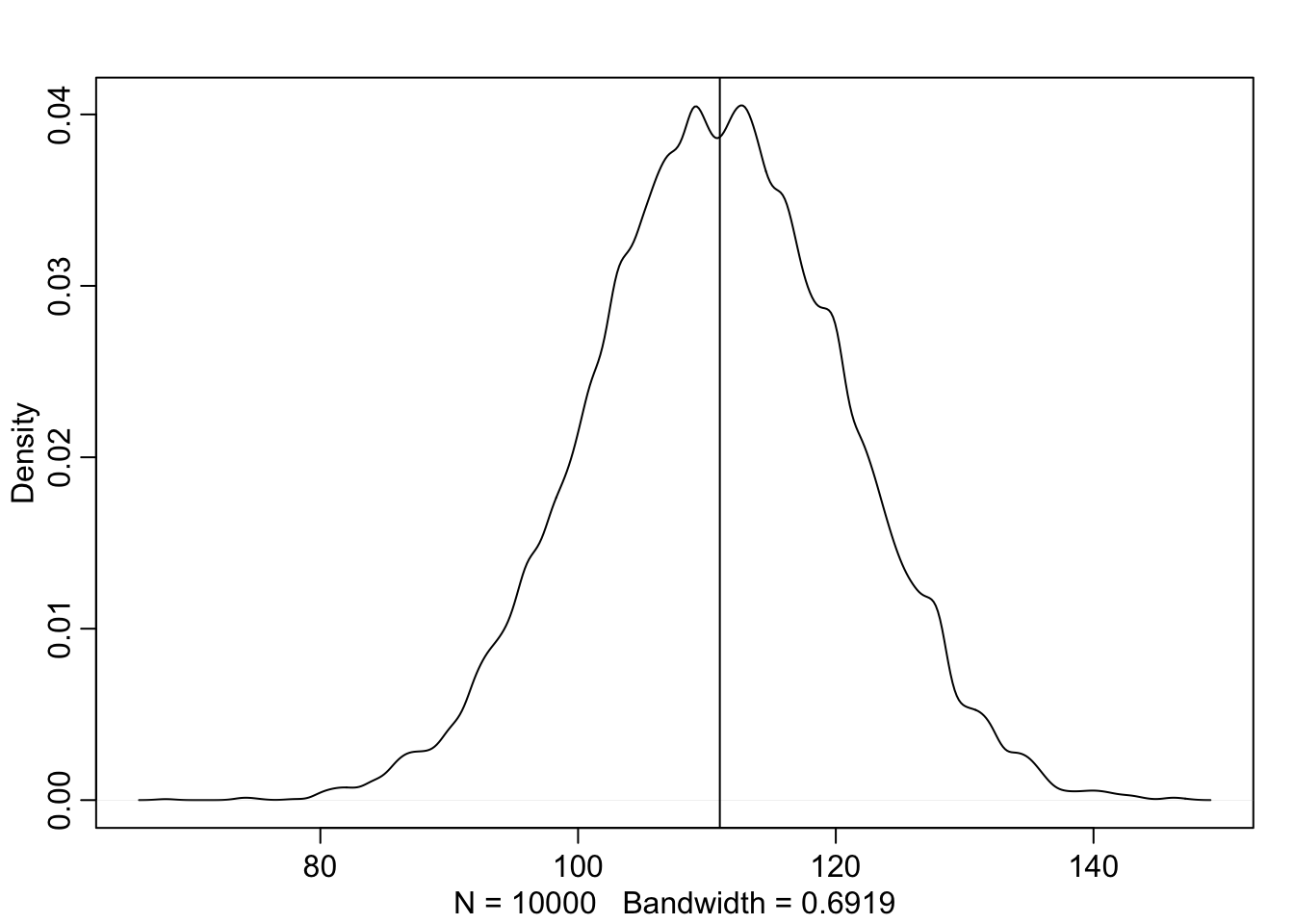
3H4
Now compare 10,000 counts of boys from 100 simulated first borns only to the number of boys in the first births, birth1. How does the model look in this light?
As we can see below our model overestimates the number of boys for the first child.
w <- rbinom(1e4, size = 100, prob = samples)
dens(w)
abline(v = sum(birth1))
3H5
The model assumes that sex of first and second births are independent. To check this assumption, focus now on the second births that followed female first borns. 1) Compare 10,000 simulated counts of boys to only those second births that followed girls. 2) To do this correctly, you need to count the number of first borns who were girls and simulate that many births, 10,000 times. 3) Compare the counts of boys in your simulations to the actual observed count of boys following girls. How does the model look in this light? Any guesses what is going on in these data.
Below we can see that the our model severly underfits our data, suggesting that births are probably not independent of one another.
# Count the number of first borns who were girls
births <- birth2[birth1 == 0]
girl_first <- length(births)

w <- rbinom(1e4, size = girl_first, prob = samples)
dens(w)
abline(v = sum(births))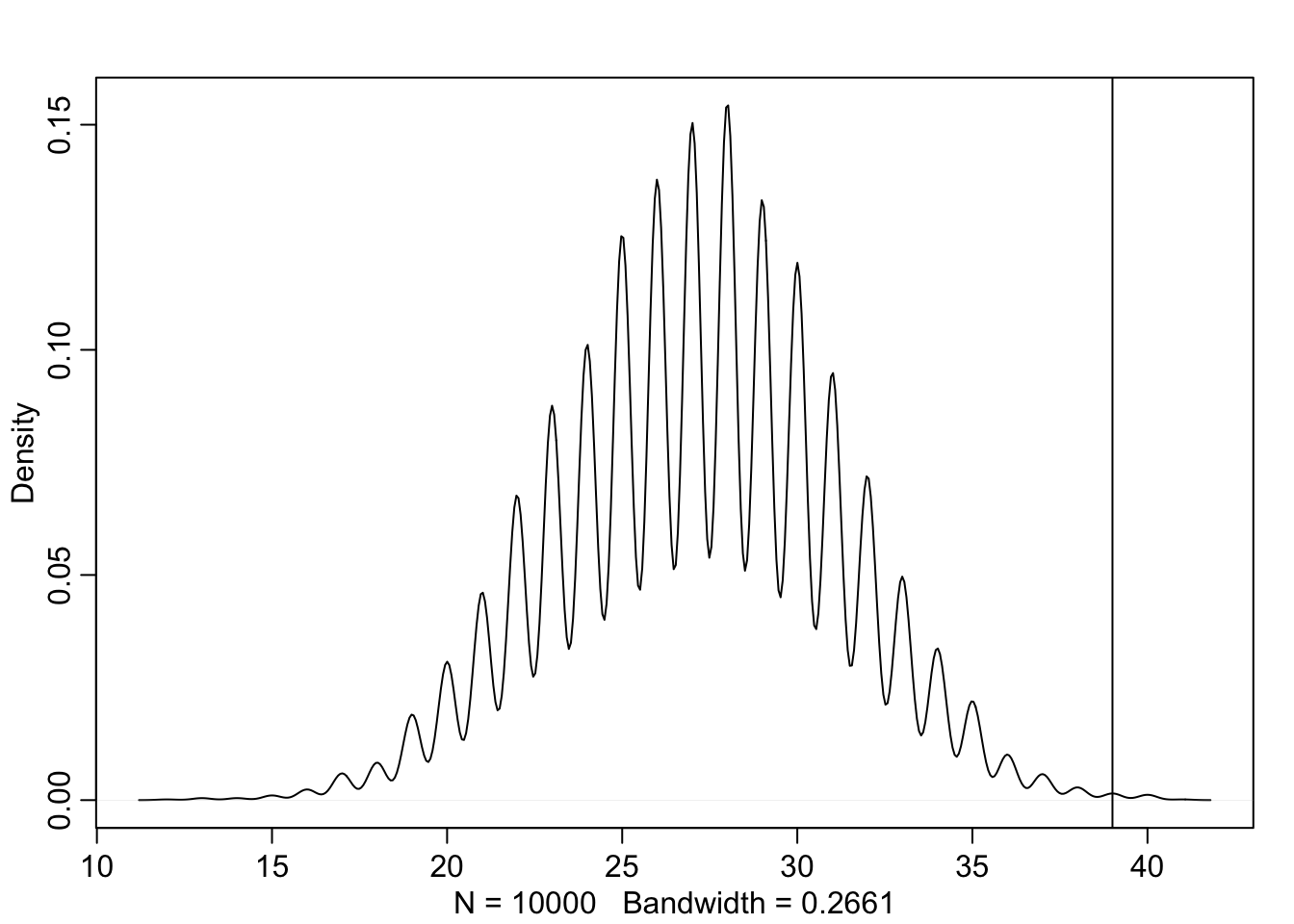
Mitchell Joseph
Data Scientist
My research interests include survival analysis, bayesian statistics, statistical learning, and finance.