Chapter 4 Problem Set
4E1
In the model definition below, which line is the likelihood? \[ \begin{array}{l} y_{i} \sim \text{Normal}(\mu, \sigma) \\ \mu \sim \text{Normal}(0, 10) \\ \sigma \sim \text{Uniform}(0, 10) \end{array} \]
In this example \(y_{i}\) is the likelihood.
4E2
In the model definition just above, how many parameters are in the posterior distribution?
In this case there are two parameters, \(\mu\) and \(\sigma\).
4E3
Using the model definition above, write down the appropriate form of Bayes’ theorem that includes the proper likelihood and prior.
Refering from page 83, we have \[ Pr(\mu,\sigma|y) = \frac{\prod_{i}\text{Normal}(y_{i}|\mu,\sigma)\text{Normal}(\mu|0,10)\text{Uniform}(\sigma|0,10)}{\int \int \prod_{i}\text{Normal}(y_{i}|\mu,\sigma)\text{Normal}(\mu|0,10)\text{Uniform}(\sigma|0,10)d\mu d\sigma} \]
4E4
In the model definition below, which line is the linear model? \[ \begin{array}{l} y_{i} \sim \text{Normal}(\mu, \sigma) \\ \mu = \alpha + \beta x_{i} \\ \alpha \sim \text{Normal}(0,10) \\ \beta \sim \text{Normal}(0,1) \\ \sigma \sim \text{Uniform}(0,10) \end{array} \] Here we have \(y_{i}\) is the likelihood, \(\alpha\), \(\beta\), and \(\sigma\) are all priors. Leaving \(\mu\) as the linear model.
4E5
In the model definition just above, how many parameters are in the posterior distribution?
We sort of answered that in the question above, it’s all the stochastic relationships, or variables defined probabilistically, read the priors. So \(\alpha\), \(\beta\), and \(\sigma\) are all the parameters in the distribution. \(\mu\) is not a parameter because it is defined deterministically instead of probabilistically.
4M1
For the model definition below, simulate observed heights from the prior (not the posterior). \[ \begin{array}{l} y_{i} \sim \text{Normal}(\mu, \sigma) \\ \mu \sim \text{Normal}(0, 10) \\ \sigma \sim \text{Uniform}(0, 10) \end{array} \]
sample_mu <- rnorm(1e4, 0, 10)
sample_sigma <- runif(1e4, 0, 10)
prior_y <- rnorm(1e4, sample_mu, sample_sigma)
dens(prior_y)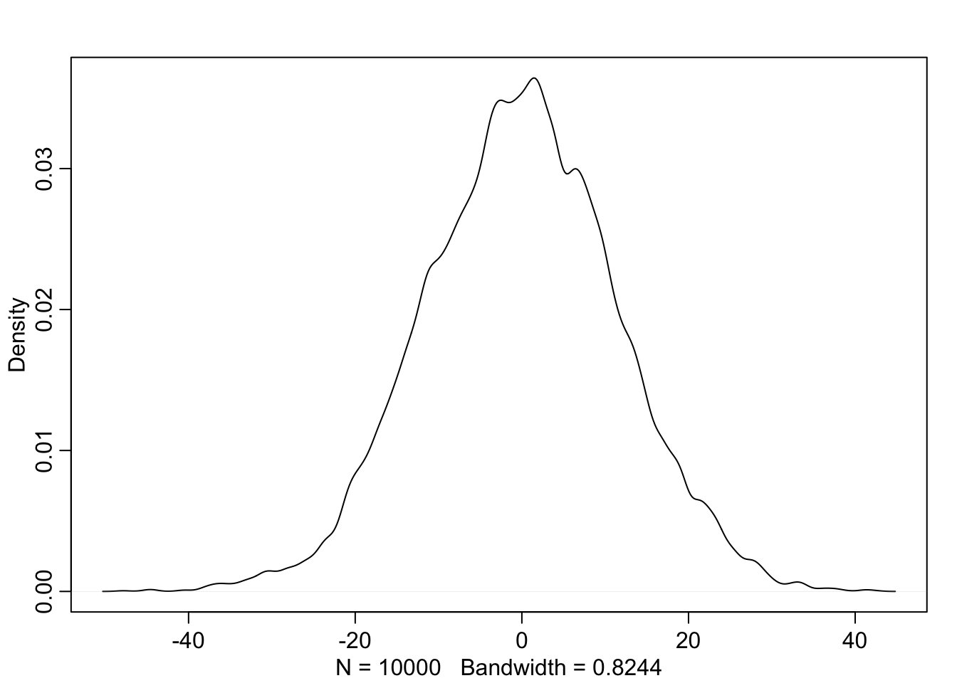
4M2
Translate the model just above into a map formula
flist <- alist(
  y ~ dnorm(mu, sigma),
  mu ~ dnorm(0, 10),
  sigma ~ dunif(0, 10)
)
4M3
Translate the map model formula below into a mathematical definition.
flist <- alist(
  y ~ dnorm(mu, sigma),
  mu <- a + b*x,
  a ~ dnorm(0, 50),
  b ~ dunif(0, 10),
  sigma ~ dunif(0, 50)
)
\[ \begin{array}{l} y_{i} \sim \text{Normal}(\mu, \sigma) \\ \mu = \alpha + \beta x_{i} \\ \alpha \sim \text{Normal}(0, 50) \\ \beta \sim \text{Uniform}(0, 10) \\ \sigma \sim \text{Uniform}(0, 50) \end{array} \]
4M4
A sample of students is measured for height each year for 3 years. After the third year, you want to fit a linear regression predicting heigh using year as a predictor. Write down the mathematical model definition for this regression, using any variable names and priors you choose. Be prepared to defend your choice of priors.
\[ \begin{array}{l} h_{i} \sim \text{Normal}(\mu, \sigma) \\ \mu = \alpha + \beta x_{i} \\ \alpha \sim \text{Normal}(140, 20) \\ \beta \sim \text{Normal}(4, 2) \\ \sigma \sim \text{Uniform}(0, 50) \end{array} \]
a <- rnorm(1e4, 140, 20)
b <- rnorm(1e4, 4, 2)
# x_i <- ceiling(runif(1e4, 0, 3))
x_i <- sample(1:3, 1e4, replace = TRUE)
# plot(x_i)
sample_mu <- a + b*x_i
sample_sigma <- runif(1e4, 0, 20)
prior_y <- rnorm(1e4, sample_mu, sample_sigma)
dens(prior_y)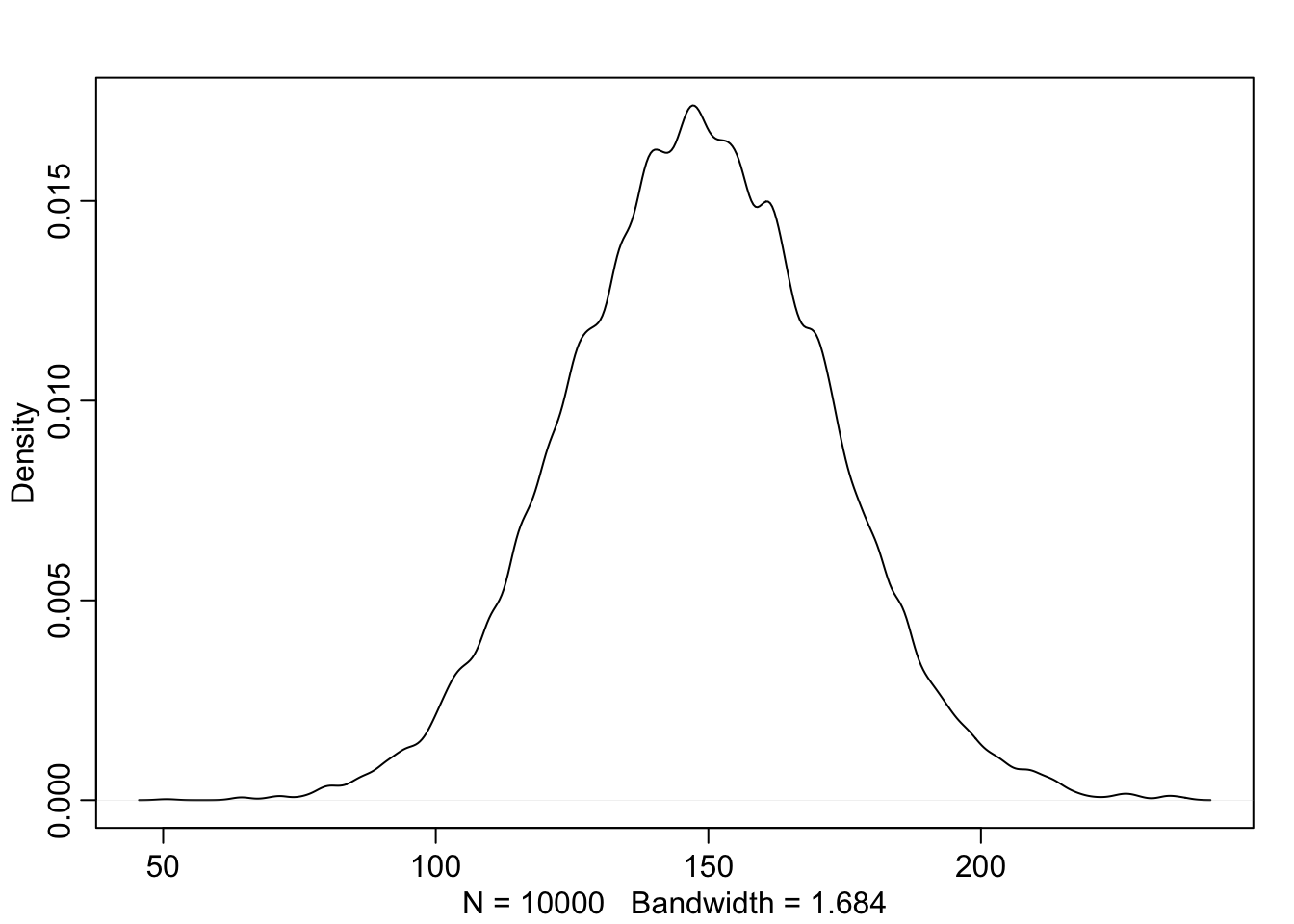
For \(\alpha\) I chose a mean of 140 because we don’t know the age of the students, and this seems like a pretty safe average, additionally, a standard deviation of 20 implies that 95% of the data will lie within the range \(140 \pm 40\). We know that most students aren’t shrinking so \(\beta\) doesn’t have to include negative values, by centering it at 4, with standard deviation of 2, we leave room for students to not grow at all, while still allowing for upwards of 8cm of growth per year which I think is adequate. \(\sigma\) was chosen to be uniformly distributed from 0 to 20 to give us a decent amount of wiggle room if needed.
4M5
Now suppose I tell you that the average height in the first year was 120cm and that every student got taller each year. Does this information lead you to change your choice of priors? How?
Yes, since the average height is 120cm we know we’re dealing with younger kids. Given this information we can center \(\alpha\) around this new average of 120cm, we’ll increase \(\beta\) because younger kids should grow more each year. Lastly, we’ll decrease sigma because we’re less likely to see children at full height. \[ \begin{array}{l} h_{i} \sim \text{Normal}(\mu, \sigma) \\ \mu = \alpha + \beta x_{i} \\ \alpha \sim \text{Normal}(120, 10) \\ \beta \sim \text{Normal}(6, 2) \\ \sigma \sim \text{Uniform}(0, 10) \end{array} \]
a <- rnorm(1e4, 120, 10)
b <- rnorm(1e4, 6, 2)
x_i <- sample(1:3, 1e4, replace = TRUE)
sample_mu <- a + b*x_i
sample_sigma <- runif(1e4, 0, 10)
prior_y <- rnorm(1e4, sample_mu, sample_sigma)
dens(prior_y)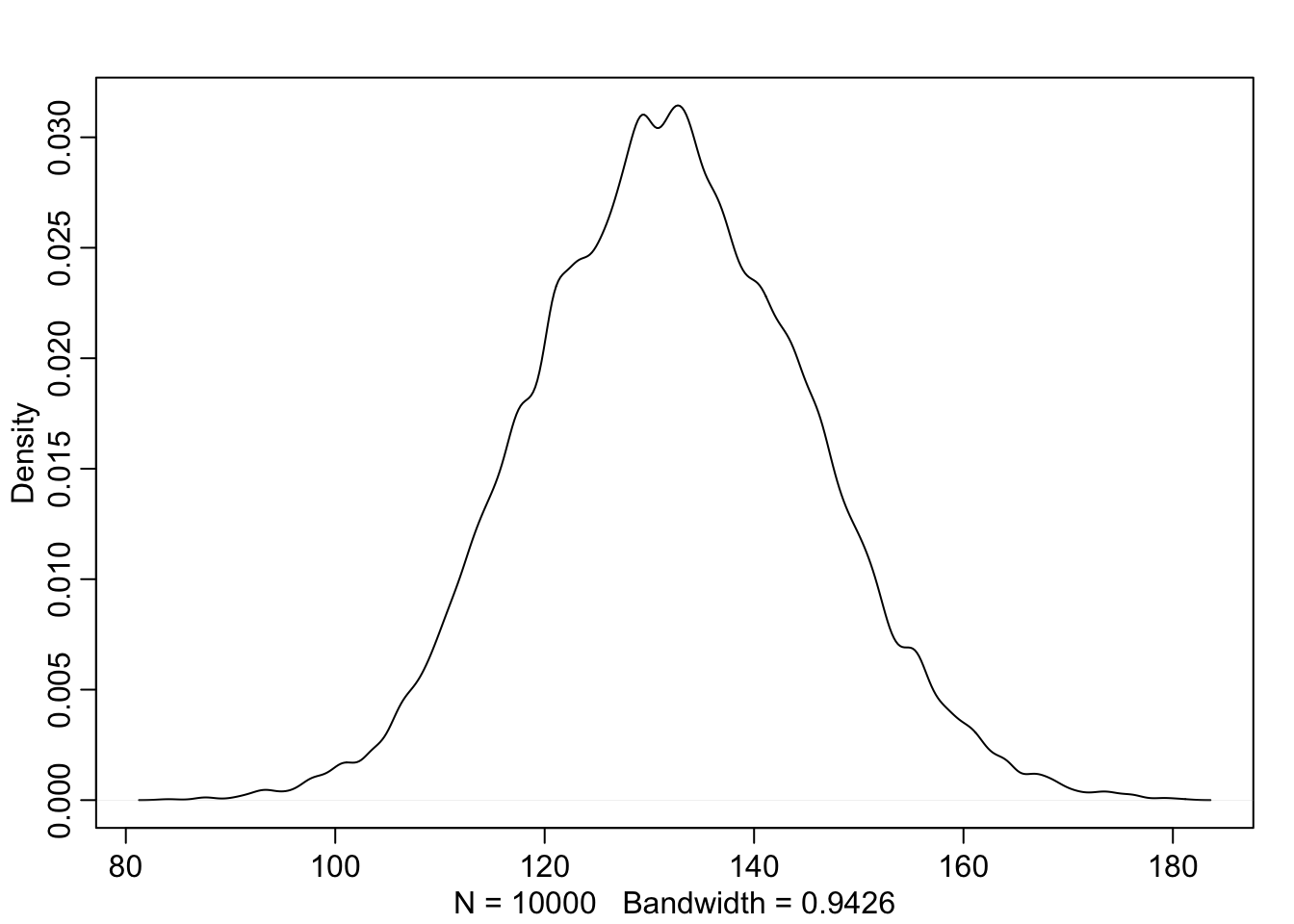
4M6
Now suppose I tell you that the variance among heights for students of the same age is never more than 64cm. How does this lead you to revise your priors?
If the variance is never more than 64cm, then the standard deviation shoudn’t be more than \(\sqrt{64} = 8\text{cm}\). We had already lowered our estimates for \(\sigma\) but we’ll just lower it slightly more.
\[ \begin{array}{l} h_{i} \sim \text{Normal}(\mu, \sigma) \\ \mu = \alpha + \beta x_{i} \\ \alpha \sim \text{Normal}(120, 10) \\ \beta \sim \text{Normal}(6, 2) \\ \sigma \sim \text{Uniform}(0, 8) \end{array} \]
4H1
the weights listed below were recorded in the !Kung census, but heights were not recorded for these individuals. Provide predicted heights and 89% intervals (either HPDI or PI) for each of these individuals. That is, fill in the table below, using model-based predictions.
| Individual | weight | expected height | 89% interval |
|---|---|---|---|
| 1 | 46.95 | ||
| 2 | 43.72 | ||
| 3 | 64.78 | ||
| 4 | 32.59 | ||
| 5 | 54.63 |
data("Howell1")
d <- Howell1
d$weight.s <- (d$weight - mean(d$weight))/sd(d$weight)
weight.seq <- c(46.95, 43.72, 64.78, 32.59, 54.63)
weight.seq.s <- (weight.seq - mean(d$weight))/sd(d$weight)

# build model
m <- quap(
  alist(
    height ~ dnorm(mu, sigma),
    mu <- alpha + beta*weight.s,
    alpha ~ dnorm(178, 100),
    beta ~ dnorm(0, 10),
    sigma ~ dunif(0, 50)
  ), data = d)

# simulate heights
sim.height <- sim(m, data = list(weight.s = weight.seq.s))

# calculate mean height and HPDI intervals
height.mean <- apply(sim.height, 2, mean)
height.HPDI <- apply(sim.height, 2, HPDI)

data.frame(cbind("expected height" = height.mean,
                 "HPDI lower" = height.HPDI[1,],
                 "HPDI upper" = height.HPDI[2,] ))
## expected.height HPDI.lower HPDI.upper
## 1 158.1460 144.1036 173.4390
## 2 152.7490 137.8508 166.2481
## 3 189.4287 174.8164 203.7536
## 4 133.4373 119.0272 148.5409
## 5 171.7682 157.8283 187.33204H2
Select out all the rows in the Howell1 data with ages below 18 years of age. If you do it right you should end up with a new data frame with 192 rows in it.
data("Howell1")
d <- Howell1 %>%
  subset(age < 18)
(a)
Fit a linear regression to these data, using map. Present and interpret the estimates. For every 10 units of increase in weight, how much taller does the model predict a child gets.
Children under the age of 18 encompass a pretty wide range of heights so I’m going to pick an \(\alpha\) that incorporates the range from 60cm to 180cm. \(\beta\) and \(\sigma\) were chosen weakly just to give ourselves enough room to work.
m <- quap(
  alist(
    height ~ dnorm(mu, sigma),
    mu <- alpha + beta * weight,
    alpha ~ dnorm(120, 30),
    beta ~ dnorm(0, 10),
    sigma ~ dunif(0, 50)
  ), data = d
)

precis(m)
## mean sd 5.5% 94.5%
## alpha 58.366630 1.39577162 56.135918 60.597343
## beta 2.714082 0.06823543 2.605028 2.823135
## sigma 8.437320 0.43058708 7.749159 9.125481We interpret this as the average height when weight is 0 is 58.37cm. For every 10 units of increase in weight, we’d expect a person to be 27.1cm taller.
(b)
Plot the raw data, with height on the vertical axis and weight on the horizontal axis. Superimpose the MAP regression line and 89% HPDI for the mean. Also superimpose the 89% HPDI for the predicted heights.
I personally prefer the graphics of ggplot, so below I used a slightly different method to that used in the book.
# model from above
m <- quap(
  alist(
    height ~ dnorm(mu, sigma),
    mu <- alpha + beta * weight,
    alpha ~ dnorm(120, 30),
    beta ~ dnorm(0, 10),
    sigma ~ dunif(0, 50)
  ), data = d
)


weight.seq <- seq(from = 0, to = max(d$weight), by = 1)
pred_dat <- list(weight = weight.seq)
mu <- link(m, data = pred_dat)
mu.mean <- apply(mu, 2, mean)
mu.HPDI <- apply(mu, 2, HPDI, prob = 0.89)
sim.height <- sim(m, data = pred_dat)
height.HPDI <- apply(sim.height, 2, HPDI, prob = 0.89)

df <- data.frame(cbind(weight.seq,
                        mu.mean,
                        "mu.lower" = t(mu.HPDI)[,1],
                        "mu.upper" = t(mu.HPDI)[,2],
                        "HPDI.lower" = t(height.HPDI)[,1],
                        "HPDI.upper" = t(height.HPDI)[,2]))

ggplot() +
  geom_ribbon(data = df,
              aes(x = weight.seq, y = mu.mean,
                  ymin = HPDI.lower, ymax = HPDI.upper),
              fill = "grey83") +
  geom_smooth(data = df,
              aes(x = weight.seq, y = mu.mean,
                  ymin = mu.lower, ymax = mu.upper),
              stat = "identity",
              fill = "grey70",
              alpha = 1,
              size = 1/2) +
  geom_point(data = d,
              aes(x = weight, y = height)) +
  coord_cartesian(xlim = range(d$weight),
                    ylim = range(d$height)) +
  labs(x = "Weight",
         y = "Height") +
  theme(panel.grid = element_blank())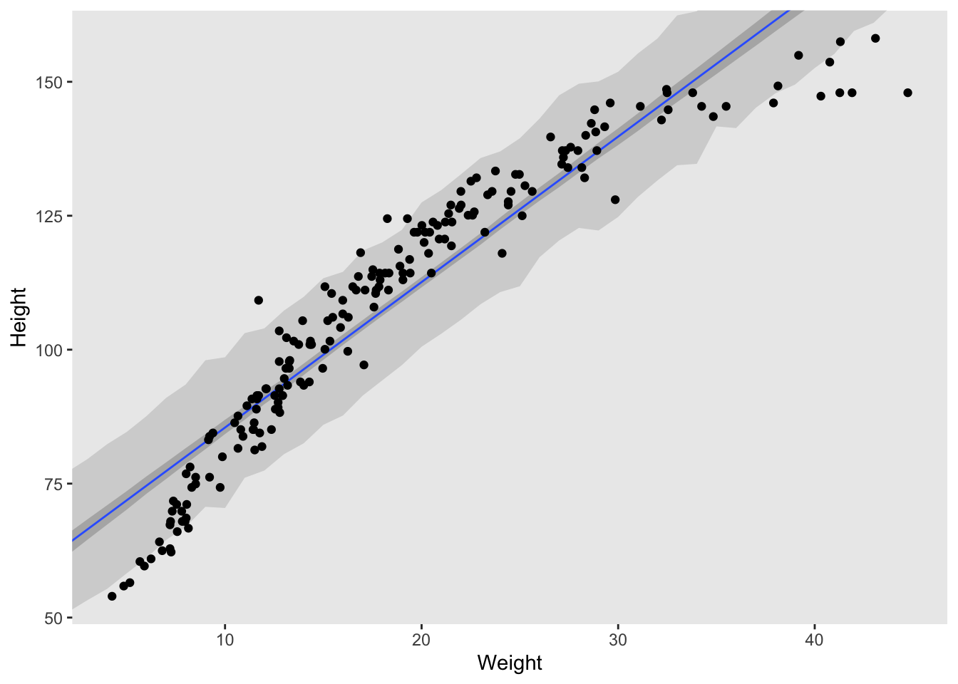
(c)
What aspects of the model fit concern you? Describe the kinds of assumptions you would change, if any, to improve the model. You don’t have to write any new code. Just explain what the model appears to be doing a bad job of, and what you hypothesize would be a better model.
The data is curved and a straight line really doesn’t fit the data very well. It’s ok for some of the middle weights but does a very poor job at either extreme. Given what we’ve learned so far, I think a second order polynomial function would be best.
4H3
Suppose a colleague of yours, who works on allometry, glances at the practice problems just above. Your colleague exclaims, “That’s silly. Everyone knows that it’s only the logarithm of body weight that scales with height!” Let’s take your colleague’s advice and see what happens.
(a)
Model the relationship between height (cm) and the natural logarithm of weight (log-kg). Use the entire Howell1 data frame, all 544 rows, adults and non-adults. Fit this model, using quadratic approximation.
\[ \begin{array}{l} h_{i} \sim \text{Normal}(\mu_{i}, \sigma) \\ \mu_{i} = \alpha + \beta\text{log}(w_{i}) \\ \alpha \sim \text{Normal}(178, 100) \\ \beta \sim \text{Normal}(0, 100) \\ \sigma \sim \text{Uniform}(0, 50) \end{array} \] where \(h_{i}\) is the height of individual \(i\) and \(w_{i}\) is the weight (in kg) of individual \(i\). The function for computing a natural log in R is just log. Can you interpret the resulting estimates?
data("Howell1")
d <- Howell1
d$weight.s <- (d$weight - mean(d$weight))/sd(d$weight)
d$weight.s2 <- d$weight.s^2

m <- quap(
  alist(
    height ~ dnorm(mu, sigma),
    mu <- alpha + beta*log(weight),
    alpha ~ dnorm(178, 100),
    beta ~ dnorm(0, 100),
    sigma ~ dunif(0, 50)
  ), data = d
)

precis(m)
## mean sd 5.5% 94.5%
## alpha -23.784150 1.3351132 -25.917919 -21.650381
## beta 47.075315 0.3825445 46.463935 47.686695
## sigma 5.134688 0.1556673 4.885902 5.383475This is a little funky to interpret to interpret.
- \(\alpha\): means that when log weight is equal to zero, height is equal to -23.78.
- \(\beta\): means that a one unit increase in log weight corresponds to a 47.08cm increase in height.
- \(\sigma\): means that the standard deviation in height predictions is 5.13cm.
(b)
Begin with this plot:
plot(height ~ weight, data=Howell1,
     col=col.alpha(rangi2, 0.4))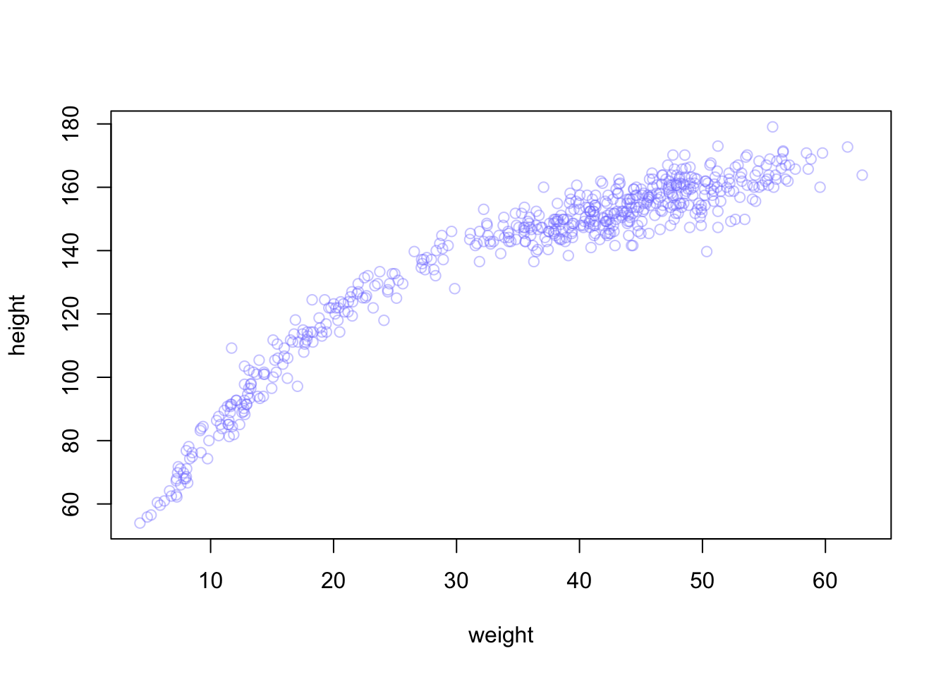
Then use samples from the quadratic approximate posterior of the model in (a) to superimpose on the plot:
- the predicted mean height as a function of weight
- the 97% HPDI for the mean
- the 97% HPDI for predicted heights
Like I mentioned before, I prefer ggplot, so things might look a little different on my end. But the code is essentially identical to part b in 4H2. The only thing we need to change is the probability ranges for our HPDI, and of course use the new model we defined in part a.
m <- quap(
  alist(
    height ~ dnorm(mu, sigma),
    mu <- alpha + beta*log(weight),
    alpha ~ dnorm(178, 100),
    beta ~ dnorm(0, 100),
    sigma ~ dunif(0, 50)
  ), data = d
)

weight.seq <- seq(from = 0, to = max(d$weight), by = 1)
pred_dat <- list(weight = weight.seq)
mu <- link(m, data = pred_dat)
mu.mean <- apply(mu, 2, mean)
mu.HPDI <- apply(mu, 2, HPDI, prob = 0.97)
sim.height <- sim(m, data = pred_dat)
height.HPDI <- apply(sim.height, 2, HPDI, prob = 0.97)

df <- data.frame(cbind(weight.seq,
                        mu.mean,
                        "mu.lower" = t(mu.HPDI)[,1],
                        "mu.upper" = t(mu.HPDI)[,2],
                        "HPDI.lower" = t(height.HPDI)[,1],
                        "HPDI.upper" = t(height.HPDI)[,2]))

ggplot() +
  geom_ribbon(data = df,
              aes(x = weight.seq, y = mu.mean,
                  ymin = HPDI.lower, ymax = HPDI.upper),
              fill = "grey83") +
  geom_smooth(data = df,
              aes(x = weight.seq, y = mu.mean,
                  ymin = mu.lower, ymax = mu.upper),
              stat = "identity",
              fill = "grey70",
              alpha = 1,
              size = 1/2) +
  geom_point(data = d,
              aes(x = weight, y = height)) +
  coord_cartesian(xlim = range(d$weight),
                    ylim = range(d$height)) +
  labs(x = "Weight",
         y = "Height") +
  theme(panel.grid = element_blank())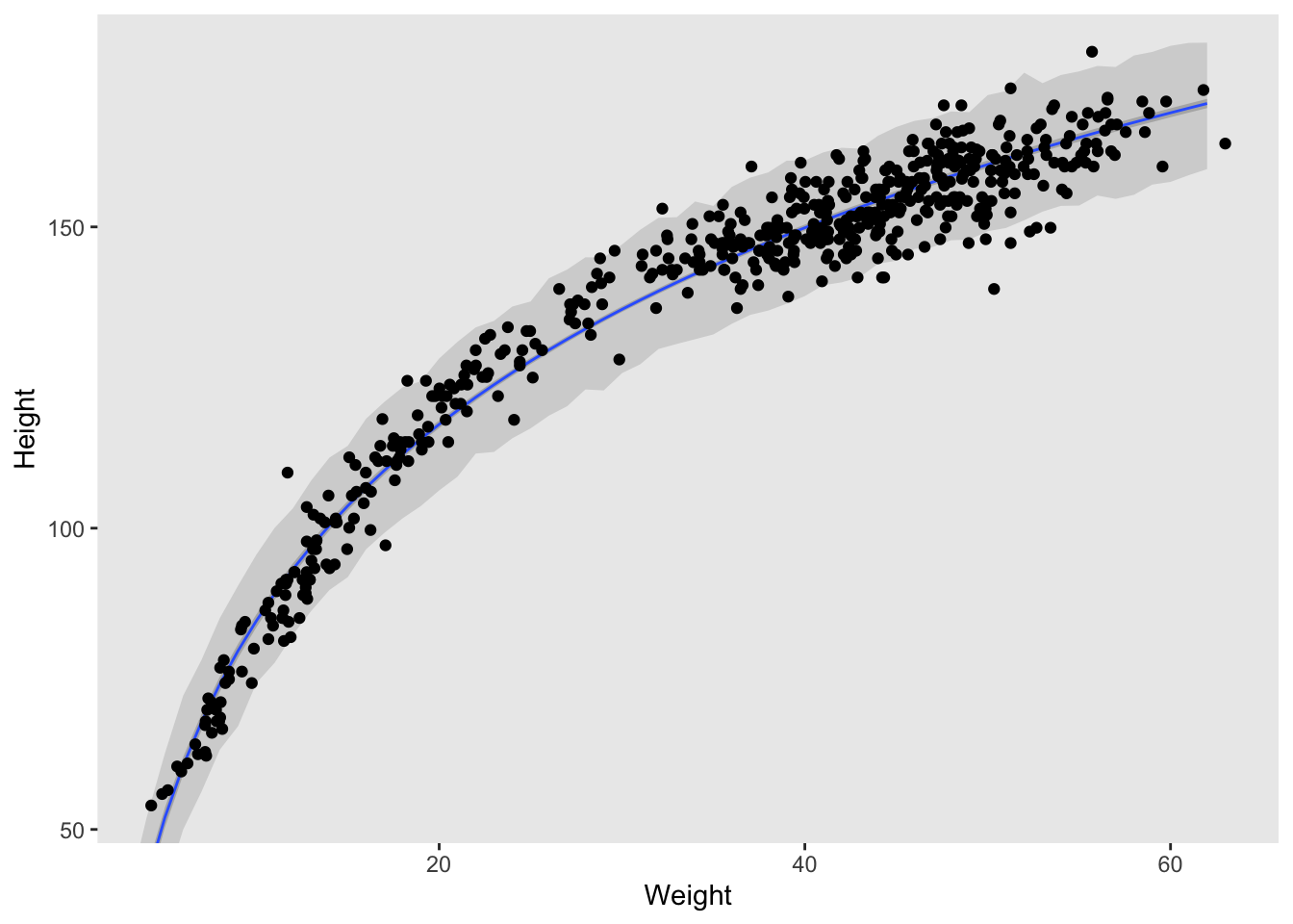
Mitchell Joseph
Data Scientist
My research interests include survival analysis, bayesian statistics, statistical learning, and finance.